Usage and Workflow
RAFT is a frequency-domain dynamics model that can be used to compute the static properties and dynamic response of a floating wind system. While it does not have any design adjustment or optimization functionalities, it is easy to interface with so that it can be used in the design loop of design and optimization tools, such as WEIS. Because of its ease of use and rapid computation time, RAFT can help design tools rapidly optimize design variables.
RAFT is run through Python, and this can be done using direction function calls or by using RAFT as part of the larger WEIS toolset. Guidance about using RAFT as part of WEIS will be provided in the WEIS documentation.
For using RAFT in a standalone capacity, the easiest way to set up a simulation is by using a YAML input file. RAFT has a defined input file format that describes simulation settings, environmental conditions, and all the necessary properties of the floating wind turbine design. This input file is discussed later on this page.
From the input file, a RAFT Model object can be generated and then interrogated to perform the RAFT analyses and extract results. The following sections discuss the process of running RAFT, the YAML input format used by RAFT, and the outputs produced by RAFT.
Running RAFT
This section discusses the relevant function calls for running RAFT independently to analyze the response of a given design across a given set of load cases. Calling these functions is also demonstrated in the example script provided on the Getting Started page.
Model Setup
A RAFT model is setup by creating a Model object based on input data contained in a Python dictionary. The dictionary can be built based off the YAML input file format described in the next section, as follows: .. code-block:
with open('VolturnUS-S_example.yaml') as file:
    design = yaml.load(file, Loader=yaml.FullLoader)  # Load the input design yaml

model = raft.Model(design)                            # Create the RAFT model
After the Model object has been made, RAFT can compute the corresponding 6-by-6 matrices for the frequency domain equations of motion (see Theory section). Then the model can be analyzed in a number of ways, the most general of which are discussed next. next.
Unloaded Condition Analysis
The model can be analyzed in its equilibrium unloaded position using the analyzeUnloaded method: .. code-block:
model.analyzeUnloaded() # Evaluate system properties and unloaded equilibrium position
This will calculate all the system’s static properties–including weight, mass, hydrostatics, and linearized mooring force and stiffness–about the system’s equilibrium position, which is also solved for in this process. It sets the RAFT Model’s states to the unloaded equilibrium position and saves these positions.
Modes and Natural Frequencies
RAFT can also perform an eigen analysis of the system to compute the rigid-body natural frequencies and mode shapes using the solveEigen method. This computation includes mooring stiffness and added mass effects.
model.solveEigen() # Evaluate system natural frequencies and mode shapes
Dynamic Load Case Analysis
The system response in all specified load cases can be analyzed using the analyzeCases method. This will run a sequence of analysis steps for each load case, first calculating any applicable mean wind load, then calculating the system mean offset, then calculating the system matrices about that mean offset, and finally solving the system dynamics in the frequency domain about that operating point.
model.analyzeCases(display=1) # Evaluate system response for each load case (and display metrics)
This method calls a number of lower-level methods in RAFT in the necessary sequence to properly evaluate each case. It
All the system static quantities are (re)evaluated
The model is analyzed for each design load cases as follows:
Linear aerodynamic and hydrodynamic properties are computed for the wind and wave conditions
The mean system offset is calculated
The mooring system is linearized about the mean offset
The aerodynamics are recomputed considering the mean pitch angle
The nonlinear properties are linearized and the full system response is calculated using an iterative process
Finally, the pertinent results are saved in a “results” dictionary that can be used for further plotting and analysis purposes (using built-in FAST functions or otherwise).
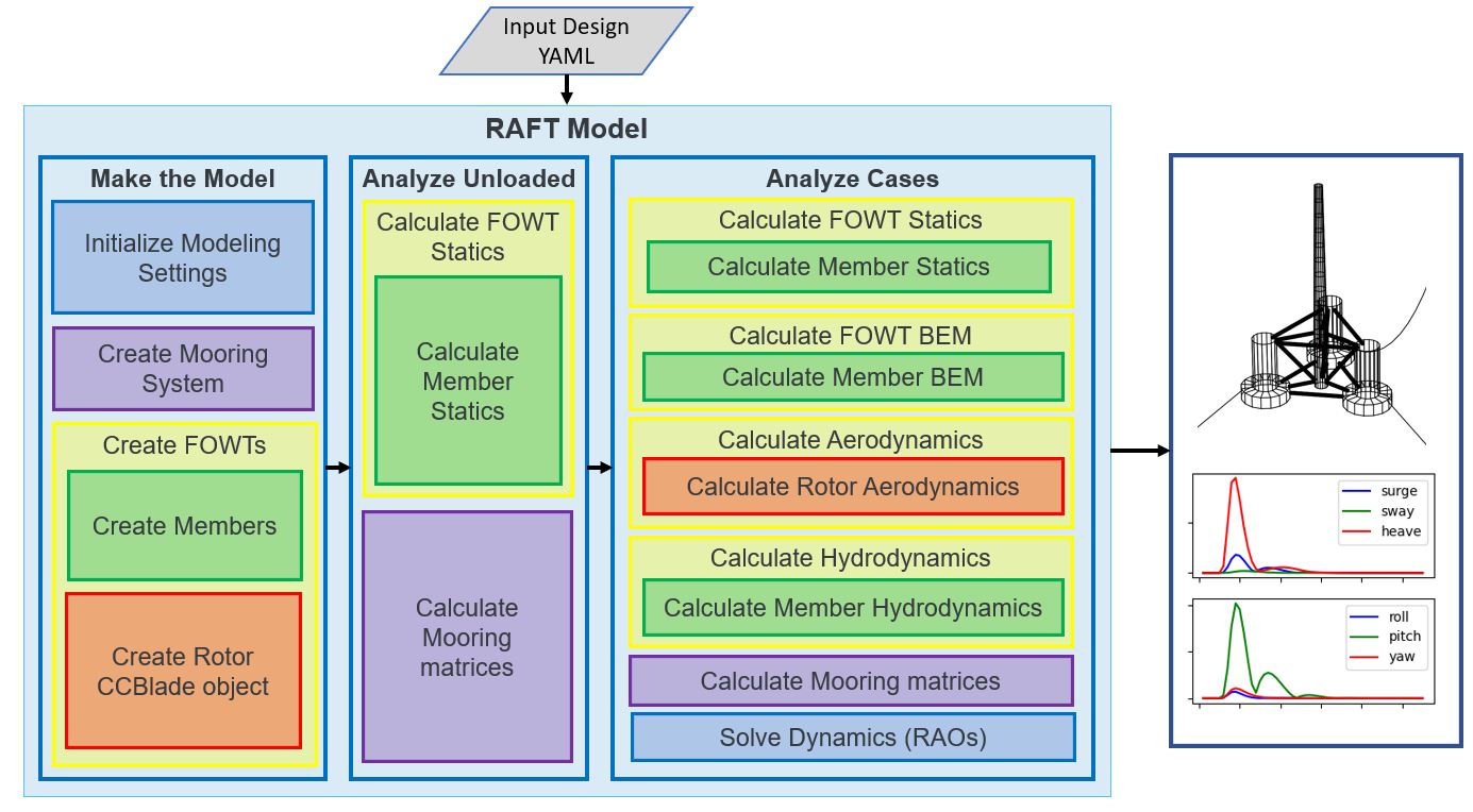
Summary
The methods described above invoke a number of lower-level methods to function, and any of these methods can be called as needed by the user in the order that suits the application. However, most applications will follow the general sequence of setup, static analysis, and dynamic analysis, which is shown in this documentation. The figure below shows this typical analysis sequence and the internal steps that are completed by RAFT to give this functionality.
Inputs
The input design YAML can be broken up into multiple parts. The following contains the various sections of an example input file for the IEA 15MW turbine with the VolturnUS-S steel semi-submersible platform.
Modeling Settings
settings:                   # global Settings
    min_freq     :  0.005   #  [Hz]       lowest frequency to consider, also the frequency bin width
    max_freq     :  0.40    #  [Hz]       highest frequency to consider
    XiStart      :   0      # sets initial amplitude of each DOF for all frequencies
    nIter        :  10      # sets how many iterations to perform in Model.solveDynamics()
    staticsMod   :   0      # sets hydrostatic stiffness approach in Model.solveStaticss (0) constant stiffness matrix or (1) nonlinear
    forcingMod   :   0      # sets forcing approach in Model.solveStatics: (0) constant or (1) updated each time
Site Characteristics
site:
    water_depth : 200        # [m]      uniform water depth
    rho_water   : 1025.0     # [kg/m^3] water density
    rho_air     : 1.225      # [kg/m^3] air density
    mu_air      : 1.81e-05   #          air dynamic viscosity
    shearExp    : 0.12       #          shear exponent
Load Cases
This section lists the environmental and operating conditions of each load case to be analyzed.
cases:
    keys : [wind_speed, wind_heading, turbulence, turbine_status, turbine_heading, wave_spectrum, wave_period, wave_height, wave_heading, current_speed, current_heading, current_turbulence  ]
    data :  #   m/s        deg    % or e.g. IIB_NTM    string            deg         string          (s)          (m)          (deg)         (m/s)           (deg)         % or e.g. IIB_NTM
        -  [     0,         0,            0,         operating,           0,        JONSWAP,         12,          1,           0,            1,              0,                   0           ]
The reference height of current_speed depends on whether it is a MHK or floating wind application. If the first (or only) rotor is underwater, then the current speed refers to the hub height of the first rotor. Otherwise, the current speed is taken to be at the water surface.
Nonzero turbine headings are not yet supported but will be in the future.
Turbine
turbine:

    mRNA          :     991000        # [kg]      RNA mass
    IxRNA         :          0        # [kg-m2]   RNA moment of inertia about local x axis (assumed to be identical to rotor axis for now, as approx) [kg-m^2]
    IrRNA         :          0        # [kg-m2]   RNA moment of inertia about local y or z axes [kg-m^2]
    xCG_RNA       :          0        # [m]       x location of RNA center of mass [m] (Actual is ~= -0.27 m)
    hHub          :        150.0      # [m]       hub height above water line [m]
    Fthrust       :       1500.0E3    # [N]       temporary thrust force to use

    I_drivetrain: 318628138.0         # [kg-m^2]  full rotor + drivetrain inertia as felt on the high-speed shaft

    nBlades     : 3                   #           number of blades
    Zhub        : 150.0               # [m]       hub height
    Rhub        : 3.97                # [m]       hub radius
    precone     : 4.0                 # [deg]
    shaft_tilt  : 6.0                 # [deg]
    overhang    : 12.0313             # [m]


    blade:
        precurveTip : -4.0            # [m]
        presweepTip : 0.0             # [m]
        Rtip        : 120.97          # [m]       rotor tip radius from axis

        geometry:
        #          r        chord     theta     precurve  presweep
          - [     8.004,    5.228,    15.474,    0.035,   0.000 ]
          - [    12.039,    5.321,    14.692,    0.084,   0.000 ]
          - [    16.073,    5.458,    13.330,    0.139,   0.000 ]
          - ...
          - [   104.832,    2.464,    -2.172,   -2.523,   0.000 ]
          - [   108.867,    2.283,    -2.108,   -2.864,   0.000 ]
          - [   112.901,    2.096,    -1.953,   -3.224,   0.000 ]
          - [   116.936,    1.902,    -1.662,   -3.605,   0.000 ]

        airfoils:
        #     station(rel)  airfoil name
          - [   0.00000,   circular       ]
          - [   0.02000,   circular       ]
          - [   0.15000,   SNL-FFA-W3-500 ]
          - [   0.24517,   FFA-W3-360     ]
          - [   0.32884,   FFA-W3-330blend]
          - [   0.43918,   FFA-W3-301     ]
          - [   0.53767,   FFA-W3-270blend]
          - [   0.63821,   FFA-W3-241     ]
          - [   0.77174,   FFA-W3-211     ]
          - [   1.00000,   FFA-W3-211     ]


    airfoils:
      - name               : circular
        relative_thickness : 1.0
        data:  # alpha       c_l         c_d         c_m
          - [ -179.9087,    0.00010,    0.35000,   -0.00010 ]
          - [  179.9087,    0.00010,    0.35000,   -0.00010 ]

      - name               : SNL-FFA-W3-500
        relative_thickness : 0.5
        data:  # alpha       c_l         c_d         c_m
          - [ -179.9660,    0.00000,    0.08440,    0.00000 ]
          - [ -170.0000,    0.44190,    0.08440,    0.31250 ]
          - [ -160.0002,    0.88370,    0.12680,    0.28310 ]
          - ...
          - [  179.9660,    0.00000,    0.08440,    0.00000 ]

      - ...


    pitch_control:
      GS_Angles: [0.06019804, 0.08713416, 0.10844806, 0.12685912, ... ]
      GS_Kp: [-0.9394215 , -0.80602855, -0.69555026, -0.60254912, ... ]
      GS_Ki: [-0.07416547, -0.06719673, -0.0614251 , -0.05656651, ... ]
      Fl_Kp: -9.35
    wt_ops:
        v: [3.0, 3.266896551724138, 3.533793103448276, 3.800689655172414, ... ]
        pitch_op: [-0.25, -0.25, -0.25, -0.25, -0.25, -0.25, -0.25, -0.25, ...]
        omega_op: [2.1486, 2.3397, 2.5309,  2.722, 2.9132, 3.1043, 3.2955, ...]
    gear_ratio: 1
    torque_control:
        VS_KP: -38609162.66552
        VS_KI: -4588245.18720


    tower:
        dlsMax    :  5.0                       # maximum node splitting section amount; can't be 0

        name      :  tower                     # [-]    an identifier
        type      :  1                         # [-]
        rA        :  [ 0, 0,  15]              # [m]    end A coordinates
        rB        :  [ 0, 0, 144.582]          # [m]    and B coordinates
        shape     :  circ                      # [-]    circular or rectangular
        gamma     :  0.0                       # [deg]  twist angle about the member's z-axis

        stations  :  [ 15,  28,  ...  144.5]   # [-]    location of stations along axis. Will be normalized such that start value maps to rA and end value to rB
        d         :  [ 10,  9.9, ...  6.5 ]    # [m]    diameters if circular or side lengths if rectangular (can be pairs)
        t         :  [ 0.08295,  0.0829,...]   # [m]    wall thicknesses (scalar or list of same length as stations)
        Cd        :  0.0                       # [-]    transverse drag coefficient       (optional, scalar or list of same length as stations)
        Ca        :  0.0                       # [-]    transverse added mass coefficient (optional, scalar or list of same length as stations)
        rho_shell :  7850                      # [kg/m3]   material density
Platform
platform:
    intersectMesh :  1       # [int] 0 for disabling and 1 for enabling meshing for intersected members, make sure you install pygmsh and meshmagick before using this option
    potModMaster  :  1       # [int] master switch for potMod variables; 0=keeps all member potMod vars the same, 1=turns all potMod vars to False (no HAMS), 2=turns all potMod vars to True (no strip)
    dlsMax        :  5.0     # maximum node splitting section amount for platform members; can't be 0

    members:   # list all members here

      - name      :  center_column             # [-]    an identifier
        type      :  2                         # [-]
        rA        :  [ 0, 0, -20]              # [m]    end A coordinates
        rB        :  [ 0, 0,  15]              # [m]    and B coordinates
        shape     :  circ                      # [-]    circular or rectangular
        gamma     :  0.0                       # [deg]  twist angle about the member's z-axis
        potMod    :  True                      # [bool] Whether to model the member with potential flow (BEM model) plus viscous drag or purely strip theory
        # --- outer shell including hydro---
        stations   :  [0, 1]                    # [-]    location of stations along axis. Will be normalized such that start value maps to rA and end value to rB
        d          :  10.0                      # [m]    diameters if circular or side lengths if rectangular (can be pairs)
        t          :  0.05                      # [m]    wall thicknesses (scalar or list of same length as stations)
        extensionA :  0.0                       # [m]    length of extension on end A of the center column. This extension is to ensure a valid boolean union operation when members are intersected. This will be automatically determined when using within WEIS.
        extensionB :  0.0                       # [m]    length of extension on end B of the center column. This extension is to ensure a valid boolean union operation when members are intersected. This will be automatically determined when using within WEIS.
        Cd         :  0.8                       # [-]    transverse drag coefficient       (optional, scalar or list of same length as stations)
        Ca         :  1.0                       # [-]    transverse added mass coefficient (optional, scalar or list of same length as stations)
        CdEnd      :  0.6                       # [-]    end axial drag coefficient        (optional, scalar or list of same length as stations)
        CaEnd      :  0.6                       # [-]    end axial added mass coefficient  (optional, scalar or list of same length as stations)
        rho_shell  :  7850                      # [kg/m3]
        # --- handling of end caps or any internal structures if we need them ---
        cap_stations :  [ 0    ]               # [m]  location along member of any inner structures (in same scaling as set by 'stations')
        cap_t        :  [ 0.001  ]             # [m]  thickness of any internal structures
        cap_d_in     :  [ 0    ]               # [m]  inner diameter of internal structures (0 for full cap/bulkhead, >0 for a ring shape)

      - name      :  outer_column              # [-]    an identifier
        type      :  2                         # [-]
        rA        :  [51.75, 0, -20]           # [m]    end A coordinates
        rB        :  [51.75, 0,  15]           # [m]    and B coordinates
        heading   :  [ 60, 180, 300]           # [deg]  heading rotation of column about z axis (for repeated members)
        shape     :  circ                      # [-]    circular or rectangular
        gamma     :  0.0                       # [deg]  twist angle about the member's z-axis
        potMod    :  True                      # [bool] Whether to model the member with potential flow (BEM model) plus viscous drag or purely strip theory
        # --- outer shell including hydro---
        stations   :  [0, 1]                    # [-]    location of stations along axis. Will be normalized such that start value maps to rA and end value to rB
        d          :  12.5                      # [m]    diameters if circular or side lengths if rectangular (can be pairs)
        t          :  0.05                      # [m]    wall thicknesses (scalar or list of same length as stations)
        extensionA : 0.0                        # [m]    length of extension on end A of the outer column. This extension is to ensure a valid boolean union operation when members are intersected. This will be automatically determined when using within WEIS.
        extensionB : 0.0                        # [m]    length of extension on end B of the outer column. This extension is to ensure a valid boolean union operation when members are intersected. This will be automatically determined when using within WEIS.
        Cd         :  0.8                       # [-]    transverse drag coefficient       (optional, scalar or list of same length as stations)
        Ca         :  1.0                       # [-]    transverse added mass coefficient (optional, scalar or list of same length as stations)
        CdEnd      :  0.6                       # [-]    end axial drag coefficient        (optional, scalar or list of same length as stations)
        CaEnd      :  0.6                       # [-]    end axial added mass coefficient  (optional, scalar or list of same length as stations)
        rho_shell  :  7850                      # [kg/m3]
        # --- ballast ---
        l_fill    :  1.4                       # [m]
        rho_fill  :  5000                      # [kg/m3]
        # --- handling of end caps or any internal structures if we need them ---
        cap_stations :  [ 0    ]               # [m]  location along member of any inner structures (in same scaling as set by 'stations')
        cap_t        :  [ 0.001  ]             # [m]  thickness of any internal structures
        cap_d_in     :  [ 0    ]               # [m]  inner diameter of internal structures (0 for full cap/bulkhead, >0 for a ring shape)

      - name      :  pontoon                   # [-]    an identifier
        type      :  2                         # [-]
        rA        :  [  5  , 0, -16.5]         # [m]    end A coordinates
        rB        :  [ 45.5, 0, -16.5]         # [m]    and B coordinates
        heading   :  [ 60, 180, 300]           # [deg]  heading rotation of column about z axis (for repeated members)
        shape     :  rect                      # [-]    circular or rectangular
        gamma     :  0.0                       # [deg]  twist angle about the member's z-axis
        potMod    :  False                     # [bool] Whether to model the member with potential flow (BEM model) plus viscous drag or purely strip theory
        # --- outer shell including hydro---
        stations   :  [0, 1]                    # [-]    location of stations along axis. Will be normalized such that start value maps to rA and end value to rB
        d          :  [12.5, 7.0]               # [m]    diameters if circular or side lengths if rectangular (can be pairs)
        t          :  0.05                      # [m]    wall thicknesses (scalar or list of same length as stations)
        extensionA :  5.0                       # [m]    length of extension on end A of the pontoon. This extension is to ensure a valid boolean union operation when members are intersected. This will be automatically determined when using within WEIS.
        extensionB :  5.0                       # [m]    length of extension on end B of the pontoon. This extension is to ensure a valid boolean union operation when members are intersected. This will be automatically determined when using within WEIS.
        Cd         :  0.8                       # [-]    transverse drag coefficient       (optional, scalar or list of same length as stations)
        Ca         :  1.0                       # [-]    transverse added mass coefficient (optional, scalar or list of same length as stations)
        CdEnd      :  0.6                       # [-]    end axial drag coefficient        (optional, scalar or list of same length as stations)
        CaEnd      :  0.6                       # [-]    end axial added mass coefficient  (optional, scalar or list of same length as stations)
        rho_shell  :  7850                      # [kg/m3]
        l_fill     :  43.0                      # [m]
        rho_fill   :  1025.0                    # [kg/m3]

      - ...
Mooring
mooring:
    water_depth: 200                           # [m]       uniform water depth

    points:
        - name: line1_anchor
          type: fixed
          location: [-837, 0.0, -200.0]
          anchor_type: drag_embedment

        - name: line2_anchor
          type: fixed
          location: [418, 725, -200.0]
          anchor_type: drag_embedment

        - name: line3_anchor
          type: fixed
          location: [418, -725, -200.0]
          anchor_type: drag_embedment

        - name: line1_vessel
          type: vessel
          location: [-58,      0.0,     -14.0]

        - name: line2_vessel
          type: vessel
          location: [29,      50,     -14.0]

        - name: line3_vessel
          type: vessel
          location: [29,     -50,     -14.0]

    lines:
        - name: line1
          endA: line1_anchor
          endB: line1_vessel
          type: chain
          length: 850

        - name: line2
          endA: line2_anchor
          endB: line2_vessel
          type: chain
          length: 850

        - name: line3
          endA: line3_anchor
          endB: line3_vessel
          type: chain
          length: 850

    line_types:
        - name: chain
          diameter:         0.185
          mass_density:   685.0
          stiffness:     3270e6
          breaking_load:    1e8
          cost: 100.0
          transverse_added_mass: 1.0
          tangential_added_mass: 0.0
          transverse_drag: 1.6
          tangential_drag: 0.1

    anchor_types:
        - name: drag_embedment
          mass: 1e3
          cost: 1e4
          max_vertical_load: 0.0
          max_lateral_load: 1e5
Outputs
RAFT saves all its output data in a “results” dictionary that is a member of the Model class. These results data can be accessed directly in Python or can be seen using built-in RAFT functionality. The outputs from RAFT fall into two categories: general and load-case-specific.
General System Quantities
General system quantities include the system’s mass and moments of inertia, hydrostatic stiffnesses, natural frequencies, and unloaded equilibrium position. These are useful for rapid design checks or even use as a preprocessing step to feed system quantities to other models.
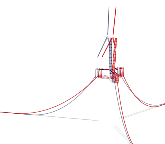
The figure below is generated by RAFT and shows the calcualted system equilibrium state in unloaded and loaded conditions (produced using the Model.plot method).
The table below shows an example of the natural frequencies and mode shapes calculated by RAFT. These are ordered as surge, sway, heave, roll, pitch, and yaw. The vectors below each natural frequency indicate the mode, which may include coupling between degrees of freedom (DOF).
Mode |
1 |
2 |
3 |
4 |
5 |
6 |
|---|---|---|---|---|---|---|
Fn (Hz) |
0.0081 |
0.0081 |
0.0506 |
0.0381 |
0.0381 |
0.0127 |
DOF 1 |
-1.0000 |
-0.0129 |
0.0000 |
0.0002 |
-0.9874 |
-0.0000 |
DOF 2 |
0.0000 |
-0.9999 |
0.0000 |
-0.9873 |
0.0001 |
0.1183 |
DOF 3 |
-0.0000 |
-0.0000 |
-1.0000 |
-0.0000 |
0.0000 |
-0.0000 |
DOF 4 |
0.0000 |
-0.0005 |
-0.0000 |
0.1586 |
-0.0000 |
0.0002 |
DOF 5 |
0.0006 |
0.0000 |
0.0000 |
0.0000 |
-0.1585 |
0.0000 |
DOF 6 |
-0.0000 |
0.0001 |
0.0000 |
0.0000 |
-0.0000 |
0.9930 |
Load-Case-Specific Outputs
The load-case-specific outputs consist of motion and load response amplitude spectra, and statistics of these responses from which mean and extreme values can be estimated. Additional calculation of fatigue loads is planned for future work.
When interfacing with RAFT, the case results can be found in ‘case_metrics’ in the Model.results data structure. Case metrics is a dictionary containing sub-dictionaries for each turbine, identified by the numbers 0 to N-1 (where N is the number of turbines). In the case of an array-level mooring system, the mooring system results will be stored at the top level. Otherwise, they will be stored individually. A partial view of the case metrics data structure is shown below. Typically, each of these entries will be an array of data, with entries corresponding to the different environmental cases.
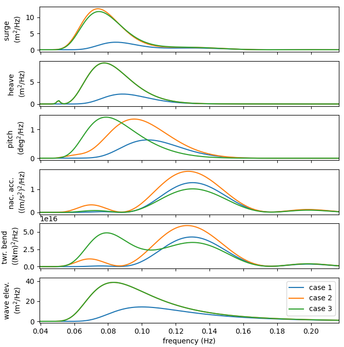
The plots below show the power spectral densities of select responses calculated from several load cases (produced using the Model.plotResponse method).
The table below shows the response statistics calculated by RAFT for an example case.
Response channel |
Average |
RMS |
Maximum |
|---|---|---|---|
surge (m) |
1.68e-02 |
6.30e-01 |
1.91e+00 |
sway (m) |
-2.54e-08 |
2.92e-09 |
-2.54e-08 |
heave (m) |
-1.34e+00 |
5.55e-01 |
3.22e-01 |
roll (deg) |
-2.88e-10 |
1.23e-09 |
3.41e-09 |
pitch (deg) |
1.16e-03 |
2.46e-01 |
7.41e-01 |
yaw (deg) |
-4.67e-12 |
2.24e-10 |
6.69e-10 |
nacelle acc. (m/s) |
0.00e+00 |
2.97e-01 |
0.00e+00 |
tower bending (Nm) |
3.69e+04 |
5.46e+07 |
0.00e+00 |
rotor speed (RPM) |
0.00e+00 |
0.00e+00 |
0.00e+00 |
blade pitch (deg) |
0.00e+00 |
0.00e+00 |
|
rotor power |
0.00e+00 |
||
line 1 tension (N) |
2.61e+06 |
3.15e+04 |
2.71e+06 |
line 2 tension (N) |
2.62e+06 |
2.45e+04 |
2.69e+06 |
line 3 tension (N) |
2.62e+06 |
2.45e+04 |
2.69e+06 |